Hi all! Do you know how to calculate percentages in Excel? In fact, percentages accompany us very often in life. After today's lesson, you will be able to calculate the profitability of an idea that suddenly arises, find out how much you actually get by participating in store promotions. Master some points and be on top of your game.
I'll show you how to use the basic calculation formula, calculate percentage growth, and other tricks.
This definition as a percentage is familiar to everyone from school. It comes from Latin and literally means “out of a hundred.” There is a formula that calculates percentages: 
Consider an example: there are 20 apples, 5 of which you gave to your friends. Determine in percentage what part did you give? Thanks to simple calculations we get the result: 
In this way, percentages are calculated both at school and in ordinary life. Thanks to Excel, such calculations become even easier, because everything happens automatically. There is no single formula for calculations. The choice of calculation method will also depend on the desired result.
How to calculate percentages in Excel: basic calculation formula
There is a basic formula that looks like:  Unlike school calculations, this formula does not need to multiply by 100. Excel takes care of this step, provided that the cells are assigned a certain percentage format.
Let's look at specific example situation. There are products that are being ordered, and there are products that have been delivered. Order in column B, named Ordered. Delivered products are located in column C named Delivered. Need to determine percentage shares of fruit delivered:
- In cell D2, write the formula =C2/B2. Decide how many rows you need and, using autocomplete, copy it.
- In the “Home” tab, find the “Number” command, select “Percent Style”.
- Look at the decimal places. Adjust their quantity if necessary.
- All! Let's look at the result.
The last column D now contains values that show the percentage of orders delivered. 
How to calculate percentages of the total amount in Excel
Now we will look at some more examples of how how to calculate percentages in excel from the total amount, which will allow you to better understand and assimilate the material.
1.The calculated amount is located at the bottom of the table
At the end of the table you can often see the “Total” cell, where the total amount is located. We have to make the calculation of each part towards the total value. The formula will look like the previously discussed example, but the denominator of the fraction will contain an absolute reference. We will have the $ sign in front of the row and column names.
Column B is filled with values, and cell B10 contains their total. The formula will look like:  Using a relative reference in cell B2 will allow it to be copied and pasted into cells in the Ordered column.
2.Parts of the amount are located on different lines
Suppose we need to collect data that is located in different rows and find out what part is taken by orders for a certain product. Adding specific values is possible using the SUMIF function. The result we get will be necessary for us to calculate the percentage of the amount.
Column A is our range, and the summing range is in column B. We enter the product name in cell E1. This is our main criterion. Cell B10 contains the total for products. The formula takes on the following form: 

In the formula itself you can place the name of the product: 
If you need to calculate, for example, how much cherries and apples occupy as a percentage, then the amount for each fruit will be divided by the total. The formula looks like this:
Calculation of percentage changes
Calculating data that changes can be expressed as a percentage and is the most common task in Excel. The formula to calculate the percentage change is as follows: 
In the process of work, you need to accurately determine which of the meanings occupies which letter. If you have more of any product today, it will be an increase, and if less, then it will be a decrease. The following scheme works:
Now we need to figure out how we can apply it in real calculations.
1.Count changes in two columns
Let's say we have 2 columns B and C. In the first we display the prices of the previous month, and in the second - this month. To calculate the resulting changes, we enter a formula in column D. 
The results of the calculation using this formula will show us whether there is an increase or decrease in price. Fill in all the lines you need with the formula using autocomplete. For formula cells, be sure to activate the percentage format. If you did everything correctly, you get a table like this, where the increase is highlighted in black and the decrease in red. 
If you are interested in changes over a certain period and the data is in one column, then we use this formula: 
We write down the formula, fill in all the lines that we need and get the following table: 
If you want to count changes for individual cells, and compare them all with one, use the already familiar absolute reference, using the $ sign. We take January as the main month and calculate the changes for all months as a percentage: 
Copying a formula across other cells will not modify it, but a relative link will change the numbering.

Calculation of value and total amount by known percentage
I have clearly demonstrated to you that there is nothing complicated in calculating percentages through Excel, as well as in calculating the amount and values when the percentage is already known.
1.Calculate the value using a known percentage
For example, you purchase new phone, which costs $950. You are aware of the VAT surcharge of 11%. It is necessary to determine the additional payment in monetary terms. This formula will help us with this: 
In our case, applying the formula =A2*B2 gives the following result: 
You can take either decimal values or using percentages.
2.Calculation of the total amount
Consider the following example, where the known original amount is $400, and the seller tells you that the price is now 30% less than last year. How to find out the original cost?
The price decreased by 30%, which means we need to subtract this figure from 100% to determine the required share: 
The formula that will determine the initial cost: 
Given our problem, we get: 

Converting a value to a percentage
This method of calculation is useful for those who especially carefully monitor their expenses and want to make some changes to them.
To increase the value by a percentage we will use the formula: 
We need to reduce the percentage. Let's use the formula: 
Using the formula =A1*(1-20%) reduces the value that is contained in a cell.
Our example shows a table with columns A2 and B2, where the first is the current expenses, and the second is the percentage by which you want to change expenses in one direction or another. Cell C2 should be filled with the formula: 

Increase by a percentage the values in a column
If you want to make changes to an entire data column without creating new columns and using an existing one, you need to do 5 steps:

Now we see values that have increased by 20%. 
Using this method, you can perform various operations on a certain percentage, entering it into a free cell.
Today was an extensive lesson. I hope you've made it clear How to calculate percentages in Excel. And, despite the fact that such calculations are not very popular for many, you will do them with ease.
Interest in modern world spinning all over the place. Not a day goes by without using them. When purchasing products, we pay VAT. Having taken out a loan from a bank, we repay the amount with interest. When reconciling income, we also use percentages.
Working with percentages in Excel
Before starting work in Microsoft Excel Let's remember school math lessons where you studied fractions and percentages.
When working with percentages, remember that one percent is a hundredth (1% = 0.01).
When performing the action of adding percentages (for example, 40+10%), we first find 10% of 40, and only then add the base (40).
When working with fractions, do not forget about the basic rules of mathematics:
- Multiplying by 0.5 is equal to dividing by 2.
- Any percentage is expressed as a fraction (25%=1/4; 50%=1/2, etc.).
We count the percentage of the number
To find a percentage of a whole number, divide the desired percentage by the whole number and multiply the result by 100.
Example No. 1. There are 45 units of goods stored in the warehouse. 9 units of goods were sold in a day. How much of the product was sold as a percentage?
9 is a part, 45 is a whole. Substitute the data into the formula:
(9/45)*100=20%
In the program we do the following:
How did this happen? Having set the percentage type of calculation, the program will independently complete the formula for you and put the “%” sign. If we set the formula ourselves (with multiplication by one hundred), then there would be no “%” sign!
Example No. 2. Let's solve the inverse problem. It is known that there are 45 units of goods in the warehouse. It also states that only 20% have been sold. How many total units of the product were sold?

Example No. 3. Let's try the acquired knowledge in practice. We know the price for the product (see picture below) and VAT (18%). You need to find the VAT amount.
We multiply the price of the product by the percentage using the formula B1*18%. 
Advice! Don't forget to extend this formula to the remaining lines. To do this, grab the lower right corner of the cell and lower it to the end. This way we get an answer to several elementary problems at once.

Example No. 4. Inverse problem. We know the amount of VAT for the product and the rate (18%). You need to find the price of a product.

Add and subtract
Let's start with the addition. Let's look at the problem using a simple example:

Now let's try to subtract the percentage from the number. Having knowledge about addition, subtraction will not be difficult at all. Everything will work by replacing one sign “+” with “-”. Working formula will look like this: B1-B1*18% or B1-B1*0.18. 
Now let's find percentage of all sales. To do this, we sum up the quantity of goods sold and use the formula B2/$B$7.

These are the basic tasks we accomplished. Everything seems simple, but many people make mistakes.
Making a chart with percentages
There are several types of charts. Let's look at them separately.
Pie chart
Let's try to create a pie chart. It will display the percentage of sales of goods. First, we are looking for percentages of all sales.

Afterwards, your diagram will appear in the table. If you are not satisfied with its location, then move it by pulling it outside the diagram. 
Histogram
For this we need data. For example, sales data. To create a histogram, we need to select all numerical values (except the total) and select the histogram in the “Insert” tab. To create a histogram, we need to select all numerical values (except the total) and select the histogram in the “Insert” tab. 
Schedule
Instead of a histogram, you can use a graph. For example, a histogram is not suitable for tracking profits. It would be more appropriate to use a graph. A graph is inserted in the same way as a histogram. You need to select a chart in the “Insert” tab. Another one can be superimposed on this graph. For example, a chart with losses. 
This is where we end. Now you know how to rationally use percentages, build charts and graphs in Microsoft Excel. If you have a question that the article did not answer, write to us. We will try to help you.
Basic definitions and properties were discussed. In this section, we'll figure out how to increase or decrease a number by a few percent and look at some other issues. If all this seems obvious to you, you can immediately skip to parts 3 - 5 of this article.
How to increase the number by a few percent. Method I
Let's start with an easy example:
Example 5. The price of the shirt increased by 20%. How much does a shirt cost now, if before the price increase it cost 2,400 rubles?
1) Find 20% of the number 2400. In the first part of the article, we discussed in detail how this is done. To find 20% of 2400, you need to multiply 2400 by twenty hundredths: 2400 * 0.2 = 480.
2) The shirt cost 2400 rubles, the price increased by 480 rubles, now the shirt costs 2400 + 480 = 2880 rubles.
Answer: 2880 rub.
If we need to reduce the number by a few percent, the reasoning is similar.
Task 7. Increase the number 250 by 40%. Reduce 330 by 12%.
Task 8. The jacket cost 18,500 rubles. During the sale the price was reduced by 20%. How much does the jacket cost now?
How to increase the number by a few percent. Method II
Let's try to solve the previous problem a little faster.
During the solution, we add twenty percent to the number 2400: 2400 + 2400 * 0.2.
Let's take the common factor out of brackets and get: 2400*(1 + 0.2) = 2400*1.2.
Conclusion: to increase the number by 20%, you should multiply it by 1.2.
Now let's formulate general rule. Suppose we need to increase the number A by t%. t% of A is t hundredths. We get:
A + A ⋅ t 100 = A ⋅ (1 + t 100)
We arrive at the following general rule:
To increase the number A by t%, you need to multiply A by (1 + t 100) .
Example 6. Increase the number 120 by 17%, the number 200 by 2%, and the number 10 by 120%.
120 ⋅ (1 + 17 100) = 120 ⋅ 1,17 = 140,4 200 ⋅ (1 + 2 100) = 200 ⋅ 1,02 = 204 10 ⋅ (1 + 120 100) = 10 ⋅ 2,2 = 22
Perhaps it is not yet very noticeable how much simpler and faster method No. 2 is compared to method No. 1. At the end of this part of the article we will look at solving the problem where the advantages of the second method will become obvious. And now - another task for independent work.
Task 9. Increase the number 1200 by 4%, the number 12 by 230%, and the number 57 by 30%.
How to reduce a number by a few percent
Literally repeating the reasoning from the previous paragraph verbatim, we arrive at the following rule:
To decrease the number A by t%, you need to multiply A by (1 − t 100) .
Example 7. There were 30 mosquitoes in the room at night. By morning their number had decreased by 40%. How many mosquitoes are left in the room?
We must reduce the number by 40%, i.e. multiply 30 by (1 − 40 100) = 1 − 0.4 = 0.6.
30*0,6 = 18.
Answer: 18 mosquitoes.
Task 10. Reduce the number 12 by 20%, reduce the number 14290 by 95%.
Twice 10% is not 20%!
Example 8. Two jackets cost 14,000 rubles each. The price of one of them was increased by 10%, and then by another 10%. The price of the second jacket was immediately increased by 20%. Which jacket costs more now?
"Why does one of them have to be more expensive?" - the reader asks in bewilderment. - “The jackets cost the same, 20% is two times 10%, which means now they also cost the same.”
Let's try to understand the situation. The first jacket increased in price by 10% twice, i.e. its cost increased twice by 1.1 times. Result: 14000*1.1*1.1 = 16940 (r). The second jacket immediately increased in price by 20%, its price was increased by 1.2 times. We calculate: 14000 * 1.2 = 16800. As you can see, the prices turned out to be different, the first jacket has risen in price more.
"But why doesn't 10% + 10% equal 20%?" - you ask.
The problem is that 10% the first time is taken from 14,000 rubles, and the second time - from the increased price.
10% of 14000r = 1400r. After the first price increase, the jacket costs 14,000 + 1,400 = 15,400 (r). Now we are rewriting the price tag again. We take 10%, but not from 14000, but from 15400: 15400*0.1 = 1540 (r). We add 1540 and 15400 - we get the final price of the jacket - 16940 rubles.
Task 11. If the starting price of the jacket were different, would the answer be different? Think about this question: take several starting price options, do the calculations. Try to prove that two 10% price increases always lead to a higher price than one 20% increase.
They raised the price by 20%, then reduced it by 20%. Back to original price?
Example 9. Actually, the task is already stated in the title. To make it easier to reason, let's modernize it a little. The jacket costs 16,000 rubles. The price was increased by 20%, and the next day - reduced by 20%. Is it true that now the jacket costs 16,000 rubles again?
No, that's not true. Short solution: 16000 * 1.2 * 0.8 = 15360 rubles - the price of the jacket has decreased.
Long solution. First, the price of the jacket increased by 20%, i.e. by 16000 * 0.2 = 3200 rubles. On the new price tag - 16000 + 3200 = 19200 (r). The next day the price is reduced by 20%. But this is already 20% not of 16,000, but of 19,200: 0.2 * 19,200 = 3,840 rubles. 19200 - 3840 = 15360 (r).
It is clear why in the end the price became lower: 20% of 19,200 is more than 20% of 16,000.
Again, I encourage you to think about how the answer would be different if the initial price of the jacket was different? Conduct several experiments: take different initial prices, carry out calculations and make sure that the final price is lower, and always by the same percentage. Can you solve this problem in general view, i.e. find out by what percentage the price of the jacket will decrease after a successive 20% increase and 20% decrease? Try it! If you can't do it yourself, look at part 3 of this article.
Several price tag changes
Example 10. In January, the cost of an apartment in a new building was 12,000,000 rubles. In February it increased by 5%, in March it decreased by 3%, in April it increased again by 7%, and in May it decreased by 10%. How much does an apartment cost now?
Solution. I hope that young mathematicians, armed with the experience of Examples 8 and 9, will not argue that the price has changed by 5% - 3% + 7% - 10% = -1%. This is a big mistake! The price changes each time from a new amount, so you can’t just add or subtract in the hope of getting the final change as a percentage.
Let me give you a detailed solution first.
The first price increase is 5% of 12,000,000 = 600,000 (r).
12,000,000 + 600,000 = 12,600,000 (r).
The first price reduction is 3% of 12,600,000 = 378,000 (r).
12,600,000 - 378,000 = 12,222,000 (r).
The second price increase is 7% of 12,222,000 = 855,540 (r).
12,222,000 + 855,540 = 13,077,540 (r).
The final price reduction by 10% is 10% of 1,307,7540 = 1,307,754 (r).
13 077 540 - 1 307 754 = 11 769 786.
Phffff, exhale!
Do you like this solution? No to me! Why these 8 actions if everything can be fit in one line:
12,000,000*1.05*0.97*1.07*0.9 = 11,769,786 (r).
I specifically included these two solutions so that you realize how much easier it is to use compared to . Unfortunately, schoolchildren rarely use the second method, preferring long arguments, like those we cited above. We need to gradually give up this bad habit!
Test No. 2
You are again offered a short test. Let me remind you that the answer (as on the Unified State Examination in mathematics) is an integer or a finite number decimal. Always use a comma as a decimal separator (for example, 1.2, but not 1.2!) Good luck!
Instructions
Let's say you need to add a fixed percentage to the original number placed in cell A1 and display the result in cell A2. Then a formula should be placed in A2 that increases the value from A1 by a certain factor. Start by determining the value of the multiplier - add one hundredth of a fixed percentage to one. For example, if you need to add 25% to the number in cell A1, then the multiplier will be 1 + (25/100) = 1.25. Click A2 and type the desired formula: enter the equal sign, click cell A1, click (multiplication sign) and type the factor. The entire entry for the example above should look like this: =A1*1.25. Press Enter and Excel will calculate and display the result.
If you need to calculate the same percentage of the values in each cell of a certain column and add the resulting value to the same cells, then place the multiplier in a separate cell. Let's say you need to add 15%, and the original values occupy the first to twentieth lines in column A. Then place the value 1.15 (1 + 15/100) in a free cell and copy it (Ctrl + C). Then select the range from A1 to A20 and press the keyboard shortcut Ctrl + Alt + V. The Paste Special dialog will appear on the screen. In the “Operation” section, check the box next to “multiply” and click the OK button. After this, all selected cells will change by the specified percentage value, and the auxiliary cell containing the multiplier can be deleted.
If it is necessary to be able to change the added percentage, it is better to place it in a separate cell, rather than correct it every time. For example, place the original value in the first line of the first column (A1), and the percentage that needs to be added in the second column of the same line (B1). To display the result in cell C1, enter the following formula into it: =A1*(1+B1/100). After pressing the Enter key, the searched value will appear in the column if cells A1 and B1 already contain required values.
Sources:
- how to add cells in excel
- Solution complex tasks on interest
In a Microsoft Office application, you can perform the same action in several ways. It all depends on what will be more convenient for the user. To add a cell to a sheet, you can choose the method that suits you.
Instructions
To add a new cell, place the cursor in the one above which you plan to add another one. Open the “Home” tab and click on the “Insert” button in the “ Cells" If you select several cells horizontally and press the same button, the same number of cells will be added above as were selected. If you select them vertically, new cells will be added to the left of the selected range.
To more accurately indicate where the additional cell should be located, place the cursor in the one near which you want to add a new one and right-click in it. In the context menu, select the second one from the top of the two “Insert” commands. A new dialog box will appear. Place a marker in it opposite one of the options: “ Cells, shifted to the right" or " Cells, with a downward shift." Click on the OK button. If you select several cells at once, the same number of new ones will be added.
The same actions can be performed using the buttons on the toolbar. Select one or more cells and click under " Cells» not the “Insert” button itself, but the arrow-shaped button located next to it. A context menu will open, select “Insert Cells” from it. After this, the same window that was discussed in the second step will appear. Select the option for adding cells that suits you and click OK.
If you designed your table using the Table tool, you will only be able to add new rows or columns. To be able to insert an empty cell, right-click in the table, select the “Table” item in the context menu and the “Convert to range” sub-item. Confirm your actions in the request window. The table view will change, after which you can insert a cell using one of the methods described above.
During calculations, sometimes you need to add percentages to a specific number. For example, to find out the current profit indicators, which have increased by a certain percentage compared to the previous month, you need to add this percentage to the profit of the previous month. There are many other examples where you need to perform a similar action. Let's figure out how to add a percentage to a number in Microsoft Excel.
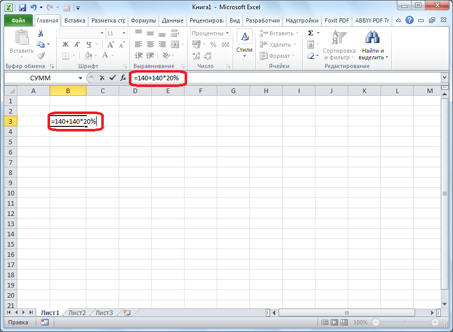
So, if you just need to find out what a number will be equal to after adding a certain percentage to it, then you should enter an expression using the following template in any cell of the sheet, or in the formula bar: “=(number)+(number)*(percentage_value )%".
Let's say we need to calculate what number we get if we add twenty percent to 140. Write the following formula in any cell, or in the formula bar: “=140+140*20%”.

Applying a formula to actions in a table
Now, let's figure out how to add a certain percentage to the data that is already in the table.
First of all, select the cell where the result will be displayed. We put a “=” sign in it. Next, click on the cell containing the data to which the percentage should be added. We put the “+” sign. Again, click on the cell containing the number and put the “*” sign. Next, we type on the keyboard the percentage by which the number should be increased. Don’t forget to put the “%” sign after entering this value.

Click on the ENTER button on the keyboard, after which the calculation result will be shown.

If you want to extend this formula to all values of a column in the table, then simply stand on the lower right edge of the cell where the result is displayed. The cursor should turn into a cross. Click on the left mouse button, and with the button held down, “stretch” the formula down to the very end of the table.

As you can see, the result of multiplying numbers by a certain percentage is also displayed for other cells in the column.

We found that adding a percentage to a number in Microsoft Excel is not that difficult. However, many users do not know how to do this and make mistakes. For example, the most common mistake is to write a formula using the algorithm “=(number)+(percentage_value)%” instead of “=(number)+(number)*(percentage_value)%”. This guide should help you avoid such mistakes.