To do this, use graph paper or a graphing calculator. Select any number of numeric values for the independent variable x (\displaystyle x) and plug them into the function to calculate the values for the dependent variable y (\displaystyle y) . Plot the found coordinates of the points on coordinate plane, and then connect these points to graph the function.
- Substitute positive numeric values x (\displaystyle x) and corresponding negative numeric values into the function. For example, given the function . Substitute it in following values x (\displaystyle x) :
- f (1) = 2 (1) 2 + 1 = 2 + 1 = 3 (\displaystyle f(1)=2(1)^(2)+1=2+1=3) (1 , 3) (\ displaystyle (1,3)) .
- f (2) = 2 (2) 2 + 1 = 2 (4) + 1 = 8 + 1 = 9 (\displaystyle f(2)=2(2)^(2)+1=2(4)+1 =8+1=9) . We got a point with coordinates (2, 9) (\displaystyle (2,9)).
- f (− 1) = 2 (− 1) 2 + 1 = 2 + 1 = 3 (\displaystyle f(-1)=2(-1)^(2)+1=2+1=3) . We got a point with coordinates (− 1, 3) (\displaystyle (-1,3)) .
- f (− 2) = 2 (− 2) 2 + 1 = 2 (4) + 1 = 8 + 1 = 9 (\displaystyle f(-2)=2(-2)^(2)+1=2( 4)+1=8+1=9) . We got a point with coordinates (− 2, 9) (\displaystyle (-2,9)) .
Check whether the graph of the function is symmetrical about the Y axis. By symmetry we mean the mirror image of the graph about the y-axis. If the part of the graph to the right of the Y-axis (positive values of the independent variable) is the same as the part of the graph to the left of the Y-axis (negative values of the independent variable), the graph is symmetrical about the Y-axis. If the function is symmetrical about the y-axis, the function is even.
- You can check the symmetry of the graph using individual points. If the value of y (\displaystyle y) x (\displaystyle x) matches the value of y (\displaystyle y) that matches the value of − x (\displaystyle -x) , the function is even. In our example with the function f (x) = 2 x 2 + 1 (\displaystyle f(x)=2x^(2)+1) we got the following coordinates of the points:
- (1.3) and (-1.3)
- (2.9) and (-2.9)
- Note that for x=1 and x=-1 the dependent variable is y=3, and for x=2 and x=-2 the dependent variable is y=9. Thus the function is even. In fact, to accurately determine the form of the function, you need to consider more than two points, but the described method is a good approximation.
Check whether the graph of the function is symmetrical about the origin. The origin is the point with coordinates (0,0). Symmetry about the origin means that a positive y value (for a positive x value) corresponds to a negative y value (for a negative x value), and vice versa. Odd functions have symmetry about the origin.
- If we substitute several positive and corresponding negative values x (\displaystyle x) , the values of y (\displaystyle y) will differ in sign. For example, given a function f (x) = x 3 + x (\displaystyle f(x)=x^(3)+x) . Substitute several values of x (\displaystyle x) into it:
- f (1) = 1 3 + 1 = 1 + 1 = 2 (\displaystyle f(1)=1^(3)+1=1+1=2) . We got a point with coordinates (1,2).
- f (− 1) = (− 1) 3 + (− 1) = − 1 − 1 = − 2 (\displaystyle f(-1)=(-1)^(3)+(-1)=-1- 1=-2)
- f (2) = 2 3 + 2 = 8 + 2 = 10 (\displaystyle f(2)=2^(3)+2=8+2=10)
- f (− 2) = (− 2) 3 + (− 2) = − 8 − 2 = − 10 (\displaystyle f(-2)=(-2)^(3)+(-2)=-8- 2=-10) . We got a point with coordinates (-2,-10).
- Thus, f(x) = -f(-x), that is, the function is odd.
Check if the graph of the function has any symmetry. The last type of function is a function whose graph has no symmetry, that is, there is no mirror image both relative to the ordinate axis and relative to the origin. For example, given the function .
- Substitute several positive and corresponding negative values of x (\displaystyle x) into the function:
- f (1) = 1 2 + 2 (1) + 1 = 1 + 2 + 1 = 4 (\displaystyle f(1)=1^(2)+2(1)+1=1+2+1=4 ) . We got a point with coordinates (1,4).
- f (− 1) = (− 1) 2 + 2 (− 1) + (− 1) = 1 − 2 − 1 = − 2 (\displaystyle f(-1)=(-1)^(2)+2 (-1)+(-1)=1-2-1=-2) . We got a point with coordinates (-1,-2).
- f (2) = 2 2 + 2 (2) + 2 = 4 + 4 + 2 = 10 (\displaystyle f(2)=2^(2)+2(2)+2=4+4+2=10 ) . We got a point with coordinates (2,10).
- f (− 2) = (− 2) 2 + 2 (− 2) + (− 2) = 4 − 4 − 2 = − 2 (\displaystyle f(-2)=(-2)^(2)+2 (-2)+(-2)=4-4-2=-2) . We got a point with coordinates (2,-2).
- According to the results obtained, there is no symmetry. The values of y (\displaystyle y) for opposite values of x (\displaystyle x) are not the same and are not opposite. Thus the function is neither even nor odd.
- Please note that the function f (x) = x 2 + 2 x + 1 (\displaystyle f(x)=x^(2)+2x+1) can be written as follows: f (x) = (x + 1) 2 (\displaystyle f(x)=(x+1)^(2)) . When written in this form, the function appears even because there is an even exponent. But this example proves that the type of function cannot be quickly determined if the independent variable is enclosed in parentheses. In this case, you need to open the brackets and analyze the obtained exponents.
Evenness and oddness of a function are one of its main properties, and parity takes up an impressive part school course in mathematics. It largely determines the behavior of the function and greatly facilitates the construction of the corresponding graph.
Let's determine the parity of the function. Generally speaking, the function under study is considered even if for opposite values of the independent variable (x) located in its domain of definition, the corresponding values of y (function) turn out to be equal.
Let's give a more strict definition. Consider some function f (x), which is defined in the domain D. It will be even if for any point x located in the domain of definition:
- -x (opposite point) also lies in this scope,
- f(-x) = f(x).
From the above definition follows the condition necessary for the domain of definition of such a function, namely, symmetry with respect to the point O, which is the origin of coordinates, since if some point b is contained in the domain of definition of an even function, then the corresponding point b also lies in this domain. From the above, therefore, the conclusion follows: the even function has a form symmetrical with respect to the ordinate axis (Oy).
How to determine the parity of a function in practice?
Let it be specified using the formula h(x)=11^x+11^(-x). Following the algorithm that follows directly from the definition, we first examine its domain of definition. Obviously, it is defined for all values of the argument, that is, the first condition is met.
The next step is to substitute the opposite value (-x) for the argument (x).
We get:
h(-x) = 11^(-x) + 11^x.
Since addition satisfies the commutative (commutative) law, it is obvious that h(-x) = h(x) and the given functional dependence is even.
Let's check the parity of the function h(x)=11^x-11^(-x). Following the same algorithm, we get that h(-x) = 11^(-x) -11^x. Taking out the minus, in the end we have
h(-x)=-(11^x-11^(-x))=- h(x). Therefore, h(x) is odd.
By the way, it should be recalled that there are functions that cannot be classified according to these criteria; they are called neither even nor odd.
Even functions have a number of interesting properties:
- as a result of adding similar functions, they get an even one;
- as a result of subtracting such functions, an even one is obtained;
- even, also even;
- as a result of multiplying two such functions, an even one is obtained;
- as a result of multiplying odd and even functions, an odd one is obtained;
- as a result of dividing the odd and even functions, an odd one is obtained;
- the derivative of such a function is odd;
- If you square an odd function, you get an even one.
The parity of a function can be used to solve equations.
To solve an equation like g(x) = 0, where the left side of the equation is an even function, it will be quite enough to find its solutions for non-negative values of the variable. The resulting roots of the equation must be combined with the opposite numbers. One of them is subject to verification.
This is also successfully used to solve non-standard problems with a parameter.
For example, is there any value of the parameter a for which the equation 2x^6-x^4-ax^2=1 will have three roots?
If we take into account that the variable enters the equation in even powers, then it is clear that replacing x with - x given equation won't change. It follows that if a certain number is its root, then the opposite number is also the root. The conclusion is obvious: the roots of an equation that are different from zero are included in the set of its solutions “in pairs”.
It is clear that the number itself is not 0, that is, the number of roots of such an equation can only be even and, naturally, for any value of the parameter it cannot have three roots.
But the number of roots of the equation 2^x+ 2^(-x)=ax^4+2x^2+2 can be odd, and for any value of the parameter. Indeed, it is easy to check that the set of roots given equation contains solutions in pairs. Let's check if 0 is a root. When we substitute it into the equation, we get 2=2. Thus, in addition to “paired” ones, 0 is also a root, which proves their odd number.
A function is called even (odd) if for any and the equality 
 .
.
The graph of an even function is symmetrical about the axis  .
.
The graph of an odd function is symmetrical about the origin.
Example 6.2. Examine whether a function is even or odd
1)
 ;
2)
;
2) ;
3)
;
3) .
.
Solution.
1) The function is defined when  . We'll find
  .
.
Those.  . Means, this function is even.
2) The function is defined when 
Those.  . Thus, this function is odd.
3) the function is defined for , i.e. For
 ,
,
 . Therefore the function is neither even nor odd. Let's call it a function of general form.
Function  is called increasing (decreasing) on a certain interval if in this interval each higher value argument corresponds to a larger (smaller) value of the function.
Functions increasing (decreasing) over a certain interval are called monotonic.
If the function  differentiable on the interval
  and has a positive (negative) derivative
  , then the function
  increases (decreases) over this interval.
Example 6.3. Find intervals of monotonicity of functions
1)
 ;
3)
;
3) .
.
Solution.
1) This function is defined on the entire number line. Let's find the derivative.
The derivative is equal to zero if  And
And  . The domain of definition is the number axis, divided by dots
  ,
, at intervals. Let us determine the sign of the derivative in each interval.

In the interval  the derivative is negative, the function decreases on this interval.
In the interval  the derivative is positive, therefore, the function increases over this interval.
2) This function is defined if  or
or
 .
.

We determine the sign of the quadratic trinomial in each interval.
Thus, the domain of definition of the function
Let's find the derivative  ,
, , If
, If  , i.e.
  , But
, But  . Let us determine the sign of the derivative in the intervals
  .
.

In the interval  the derivative is negative, therefore, the function decreases on the interval
  . In the interval
  the derivative is positive, the function increases over the interval
  .
.
Dot  called the maximum (minimum) point of the function
  , if there is such a neighborhood of the point
  that's for everyone
  from this neighborhood the inequality holds
 .
.
The maximum and minimum points of a function are called extremum points.
If the function  at the point
  has an extremum, then the derivative of the function at this point is equal to zero or does not exist (a necessary condition for the existence of an extremum).
The points at which the derivative is zero or does not exist are called critical.
5. Sufficient conditions for the existence of an extremum.Rule 1. If during the transition (from left to right) through the critical point  derivative
  changes sign from “+” to “–”, then at the point
  function
  has a maximum; if from “–” to “+”, then the minimum; If
  does not change sign, then there is no extremum.
Rule 2. Let at the point  first derivative of a function
  equal to zero
  , and the second derivative exists and is different from zero. If
  , That
  – maximum point, if
  , That
  – minimum point of the function.
Example 6.4. Explore the maximum and minimum functions:
1)
 ;
2)
;
2) ;
3)
;
3) ;
;
4)
 .
.
Solution.
1) The function is defined and continuous on the interval  .
.
Let's find the derivative  and solve the equation
  , i.e.
  .From here
  – critical points.
Let us determine the sign of the derivative in the intervals ,  .
.

When passing through points  And
And  the derivative changes sign from “–” to “+”, therefore, according to rule 1
  – minimum points.
When passing through a point  the derivative changes sign from “+” to “–”, so
  – maximum point.
 ,
,
 .
.
2) The function is defined and continuous in the interval  . Let's find the derivative
  .
.
Having solved the equation  , we'll find
  And
And  – critical points. If the denominator
  , i.e.
  , then the derivative does not exist. So,
  – third critical point. Let us determine the sign of the derivative in intervals.

Therefore, the function has a minimum at the point  , maximum in points
  And
And  .
.
3) A function is defined and continuous if  , i.e. at
  .
.
Let's find the derivative 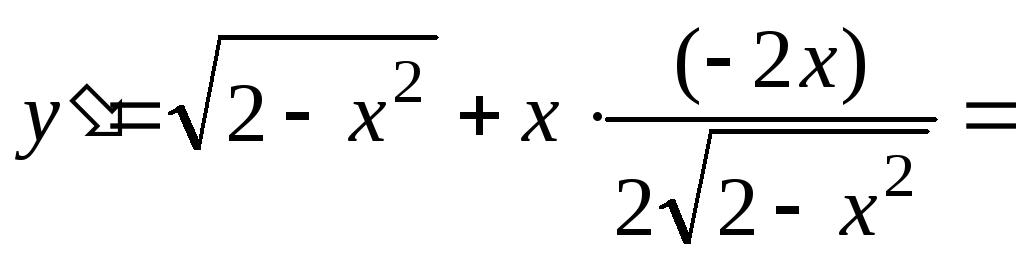
 .
.
Let's find critical points: 

Neighborhoods of points  do not belong to the domain of definition, therefore they are not extremums. So, let's examine the critical points
  And
And  .
.

4) The function is defined and continuous on the interval  . Let's use rule 2. Find the derivative
  .
.
Let's find critical points:
Let's find the second derivative  and determine its sign at the points
At points  function has a minimum.
At points  the function has a maximum.
How to insert mathematical formulas on a website?
If you ever need to add one or two mathematical formulas to a web page, then the easiest way to do this is as described in the article: mathematical formulas are easily inserted onto the site in the form of pictures that are automatically generated by Wolfram Alpha. In addition to simplicity, this universal method will help improve the visibility of the site in search engines. It has been working for a long time (and, I think, will work forever), but is already morally outdated.
If you regularly use mathematical formulas on your site, then I recommend that you use MathJax - a special JavaScript library that displays mathematical notation in web browsers using MathML, LaTeX or ASCIIMathML markup.
There are two ways to get started using MathJax: (1) using simple code you can quickly connect a MathJax script to your website, which will be automatically loaded from a remote server at the right time (list of servers); (2) download the MathJax script from a remote server to your server and connect it to all pages of your site. The second method - more complex and time-consuming - will speed up the loading of your site's pages, and if the parent MathJax server becomes temporarily unavailable for some reason, this will not affect your own site in any way. Despite these advantages, I chose the first method as it is simpler, faster and does not require technical skills. Follow my example, and in just 5 minutes you will be able to use all the features of MathJax on your site.
You can connect the MathJax library script from a remote server using two code options taken from the main MathJax website or on the documentation page:
One of these code options needs to be copied and pasted into the code of your web page, preferably between tags and or immediately after the tag. According to the first option, MathJax loads faster and slows down the page less. But the second option automatically monitors and loads the latest versions of MathJax. If you insert the first code, it will need to be updated periodically. If you insert the second code, the pages will load more slowly, but you will not need to constantly monitor MathJax updates.
The easiest way to connect MathJax is in Blogger or WordPress: in the site control panel, add a widget designed to insert third-party JavaScript code, copy the first or second version of the download code presented above into it, and place the widget closer to the beginning of the template (by the way, this is not at all necessary , since the MathJax script is loaded asynchronously). That's it. Now learn the markup syntax of MathML, LaTeX, and ASCIIMathML, and you are ready to insert mathematical formulas into your site's web pages.
Any fractal is constructed according to a certain rule, which is consistently applied an unlimited number of times. Each such time is called an iteration.
The iterative algorithm for constructing a Menger sponge is quite simple: the original cube with side 1 is divided by planes parallel to its faces into 27 equal cubes. One central cube and 6 cubes adjacent to it along the faces are removed from it. The result is a set consisting of the remaining 20 smaller cubes. Doing the same with each of these cubes, we get a set consisting of 400 smaller cubes. Continuing this process endlessly, we get a Menger sponge.