a certain quantity of a good or service offering that producers are willing to sell at a certain price over a certain period of time
Definition of supply in economics, individual and market supply, function and law of supply, supply scale and curve, supply price and pricing factors, non-price supply factors, supply elasticity, factors and types of supply elasticity, supply elasticity coefficient, taxes and supply elasticity
Expand contents
Collapse content
Supply in economics is, definition
The offer is a concept that reflects the behavior of a commodity producer in the market and an economic indicator representing market funds, and the total volume of goods in physical terms of a certain quantity or services, as well as the opportunity, ability and desire of sellers and producers, which can be offered at a specific price from a range of possible prices in a given specific sales market over a certain period of time, with constant values of other factors.
The offer is a concept that reflects the behavior of a commodity producer on the market, his willingness to produce (offer) any quantity of goods over a certain period of time under certain conditions.

The offer is economic indicator, the volume of goods in physical terms that can be offered at a specific price for this market sales for a certain period of time with constant values of other factors.

The offer is The ability and willingness of sellers to offer a certain quantity of a product at a given price.
Basic definitions of a sentence
The offer is the desire of the manufacturer to produce and offer its goods for sale on the market at specific prices from a range of possible prices for a certain time.

The offer is a certain quantity of goods that sellers wish to sell on a specific market in a given period under specific conditions.

The offer is the total quantity of any product that can be put up for sale over a certain period of time under certain conditions.

The offer is can be defined as a scale showing the different quantities of a product that a manufacturer is willing and able to produce and offer for sale in the market at any given price out of a range of possible prices over a specified period of time.

The offer is the quantity of a product that sellers want and can offer to the market in a certain period of time at all possible prices for this product.
The offer is the relationship between the quantity of a good that sellers are willing and able to sell and the prices for that good.

The offer is the quantity of a good or service supply that producers are willing to sell at a certain price during a certain period.

The offer is the quantity of goods (services) that sellers are able and willing to sell at a certain price in a given place and at a given time.

The offer is a well-formed formula that does not contain free occurrences of variables (that is, occurrences that are not within the scope of any quantifiers in the formula).

The offer is the amount of goods (services) that sellers are willing to sell on the market.

The offer is a set of goods with certain prices that are on the market (or in transit) and that producers-sellers can or intend to sell.

The offer is the relationship between the price of a good and the quantity of it that sellers are willing and able to sell.

The offer is the quantity of goods and services that sellers are willing to offer at a given price level in a certain period of time.

The offer is the desire and ability of sellers to supply goods for sale on the market. Accordingly, the volume of supply is the amount of goods that sellers are willing to produce and sell within a certain time, at a certain price.

The offer is a concept that reflects the behavior of a commodity producer on the market, his willingness to produce (offer) any quantity of goods over a certain period of time under certain conditions. The manufacturer solves two problems: how much to produce and at what price. The higher the price, the higher the supply; the lower the price, the lower the supply.

Offer- This the totality of goods on the market or capable of being delivered there is the sum of goods that sellers are willing to sell at different dynamics of the market price. In other words, the supply represents market funds, that is, the totality of goods that arrives for final sale.

Analysis of the concept of supply in economics
Supply shows what quantities of a product will be offered for sale at different prices, all other factors remaining constant. IN in this case Let's assume our producer is a potato farmer. Our definition of "supply" shows that supply is usually viewed in terms of value for money. In other words, we believe that supply indicates the quantity of a product that producers will offer at various possible prices. However, it is equally correct, and in some cases even more useful, to consider the proposal in terms of its magnitude. Instead of asking what quantities will be supplied at different prices, we are entitled to ask what prices should be that will induce the producer to offer different quantities of the good.

Supply dynamics are influenced by various factors, primarily price. The proposal should be considered in terms of its magnitude. Instead of asking what quantities will be supplied at different prices, we are entitled to ask what prices should be that will induce the producer to offer different quantities of the good. Supply is the quantity (volume) of goods offered for sale on the market at a certain point or period of time. In value terms, supply represents the sum of the market prices of these goods.

The manufacturer strives to maximize the profit he receives, i.e. the difference between the proceeds from the sale of products produced by him and the costs of its production. This means that when deciding on the volume of production to offer on the market, the manufacturer will always choose the volume of production that provides him with the greatest profit. Consequently, in order to determine the nature of the supply function on price, it is necessary to find out how the volume of production that provides the greatest profit will change when the price of the product changes (but with constant values of other factors influencing the amounts of revenue and costs).

Let us find out, first of all, what volume of production will provide the manufacturer with maximum profit at each value of the price of the product. It is obvious that each subsequent unit of production not only promises an increase in total revenue, but also requires, on the other hand, an increase in costs. In other words, producing an additional unit of output causes total revenue to increase by some amount, which economists call marginal revenue, and a simultaneous increase in total costs by an amount called marginal cost.

If the production of an additional unit of output adds to total revenue an amount greater than the amount added by producing that unit of output to total costs (i.e., marginal revenue is greater than marginal cost), then the producer's profit increases. Otherwise, when marginal revenue is less than marginal cost, profit decreases. Let us now try to determine how the relationship between marginal revenue and marginal costs changes with changes in production volume. To do this, let us consider separately how marginal revenue and marginal costs change when the volume of output changes.

The situation with marginal revenue is quite simple. Since we want to determine the volume of output characterized by the greatest profit at given value price of the product, then the price acts in this case for the manufacturer as a given value. The manufacturer believes that no matter how many units he produces, he still will not be able to influence the price. Thus, each subsequent unit of goods produced adds to total revenue the same amount equal to the price of the goods as the previous units. Marginal revenue equals price.

Before moving on to analyzing marginal costs, let's take a closer look at the production process of a product. The manufacturer, using the necessary resources, produces in some way a product that can be sold directly to the consumer.
Product manufacturing process
The term “production” is understood here in a broad sense and refers not only to industrial production, but also to trade, the service sector and, in general, any activity that transforms resources into goods needed by the consumer. Let us consider from this point of view a garment factory and a ready-made clothing store. The first, using resources such as fabric, equipment, and workers' labor, produces clothes, which from the point of view of the factory are goods, since they can be sold to the consumer - the store. However, from the point of view of the latter, clothing is a resource that, together with other resources - premises, labor of sellers, etc. - makes it possible to sell goods (clothes in a store) to the end consumer.

How does marginal cost change with changes in production volume? Let us remember that our task is to determine the nature of the supply function on price, other conditions being constant. If other conditions (i.e. resource prices, level of technology, etc.) remain unchanged, then it is obvious that the reason for any change in marginal costs should be sought in the nature of the production process itself, or more precisely, in the productivity of the resources used (factors of production ). If this productivity were a constant value, then the marginal costs in the case we are considering would be constant for any change in the volume of output. But economists believe this is not the case, basing their argument on the law of diminishing returns. Let us illustrate this law with a simple example.

Let a farmer own a plot of land of 1 hectare. Each additional quantity of potatoes grown on this plot requires additional labor. Then what will be the productivity of each subsequent unit of labor applied to the land? Economists call the marginal productivity of a factor of production the increase in output that is caused by the use of an additional unit of that factor. It can be assumed that at first the marginal productivity of labor will even increase (two people will be able to produce not twice as many potatoes as one, but even more), but it is obvious that sooner or later the marginal productivity will begin to decrease (i.e. the eleventh person will increase the total number of potatoes collected is less than a tenth, etc.).

In our example, one of the factors of production (land) acted as constant, and the other (labor) acted as variable. Note that from the point of view of an individual producer, some factors are always constant, at least in some short period, when it is impossible to quickly increase the size of a plot of land, a plant, etc. Other factors (raw materials, labor) are variable, and any change in the volume of output is associated with a change in the number of units of these factors used. Let us now formulate the law of diminishing productivity in general form: if one of the factors of production is variable and the others are constant, then, starting from a certain moment, the marginal productivity of each subsequent unit of the variable factor decreases.

What conclusion can be drawn based on the law of diminishing returns? It is quite obvious that a decrease in marginal productivity means nothing more than an increase in marginal costs. After all, if each subsequent unit of a variable factor increases the volume of output by an amount less than the previous one, then to increase the volume of production for each additional unit, an increasing number of units of the variable factor are required. Consequently, marginal cost increases, although the unit price of the variable factor remains unchanged.

Now we know how marginal revenue and marginal cost change with changes in production volume. Marginal revenue is constant and equal to price, and marginal cost first falls (as marginal productivity increases) and then begins to rise (as marginal productivity decreases). At what volume of output will the manufacturer receive maximum profit? If only the production of a given good can bring any profit at all (otherwise the good will not be produced), this profit will increase all the time while marginal costs decrease. But even when marginal costs begin to increase, profit will continue to increase for some time until marginal costs are less than marginal revenue (price of the product), i.e. The release of each subsequent unit of goods will increase total profit. Only when marginal cost exceeds marginal revenue will profits decrease as more units are produced. Thus, the greatest profit for the manufacturer will be provided by the volume of output at which marginal costs will be equal to marginal revenue, i.e. price of the goods.

So, we have established what the volume of supply of goods at a given price will be by an individual manufacturer. What happens if the price of a product changes? Obviously, an increase in price will make profitable production several additional units of a good with higher marginal costs until the marginal cost of producing the last unit equals the new price of the good. Conversely, if the price decreases, the few units with the highest marginal costs will have to be abandoned until the marginal cost returns to the new price. In other words, the quantity supplied of a good increases when the price increases and decreases when it decreases.

In economics, there are two types of supply: individual and market.

Individual offer
Individual offer - an offer from an individual manufacturer. An individual offer is corresponding to each given price, the quantity of goods that one or another manufacturer (seller) is ready to offer for sale on the market. The supply of different manufacturers (sellers) can change with varying degrees of intensity when the price changes.

The more supply changes in response to an equal change in price, the flatter the individual supply line appears on the graph. When it is positioned horizontally, the dependence of volume changes on price changes tends to infinity. On the contrary, the vertical appearance of the supply line indicates the “insensitivity” of the supply function to any price changes.

The slope of the market supply curve depends on the number of producers (sellers) and the total volume of their supply. Let's combine the supply and demand lines on one graph. The supply and demand lines intersect at point E. At E (equilibrium point), the price at which buyers are willing to buy a certain quantity of a product is equal to the price at which producers are willing to sell the same quantity of a product - it suits buyers and producers (market equilibrium). The sales volume at this point is the equilibrium market volume. The price at this point is the equilibrium (market) price. If the price prevailing on the market differs from the equilibrium price, then under the influence of market mechanisms it will change until it is established at an equilibrium level and the volume of demand becomes equal to the volume of supply. If the price on the market is higher than the equilibrium price, then the quantity demanded at this price will be less than the quantity supplied, and producers will not be able to sell all their products. There is a surplus of goods on the market. Producers will begin to reduce the price to the equilibrium price level. If the price is lower than the equilibrium price, then the volume of demand will exceed the volume of supply and a shortage of goods will form on the market. In this case, manufacturers will begin to increase the price.

Market supply is a set of individual offers for a given product. The market supply is found purely arithmetically, as the sum of offers of a given product by different producers at each possible price. The market supply schedule is determined by horizontally summing the individual supply schedules. The main factors of supply are the price of the good and non-price factors.

The transition to market supply is similar to the transition from individual to market demand. In this case, it is possible to use both methods: tabular and graphical. Let's give an example of a graphical solution. Let there be only two firms, manufacturers A and B, on the market. The dependence of their individual supply on price is presented in the first two graphs. It is easy to notice that the slope of the market supply curve depends on the number of producers (sellers) and the total volume of their supply.

The market supply curve is less steeply sloped than individual sellers' curves because the market responds to higher prices with a larger absolute increase in quantity supplied.
Market and market supply
Market offer vs individual
Just as market demand is the sum of the demands of all buyers, market supply is the sum of the offers of all sellers. The table shows the supply data at each possible price for two ice cream manufacturers - Ben and Jerry's. Market supply is the sum of these individual offers.

The volume of market supply depends on the factors that determine the supply of individual sellers: the price of the product, the price of the resources used to produce the product, the level of technology and expectations, and in addition, the number of suppliers. (If Ben or Jerry go out of business, the quantity supplied of ice cream in the market will decrease.) The supply schedule (see table) shows the change in quantity supplied as price changes, when other variables that determine it are held constant.

The figure shows supply curves constructed from the data in the table. As in the case of the demand curve, in order to obtain the market supply curve, we sum the individual supply curves horizontally. That is, to find the total quantity supplied at each possible price, we sum the individual supply along the horizontal axis of the individual demand curves. The market demand curve reflects the change in total supply in accordance with the change in the price of the product.

The supply function is dependence of the volume of market supply of an economic good on its determining factors. The function of supply is, in general terms, to link production with consumption, the sale of goods with their purchase. Reacting to emerging demand, production begins to increase the output of goods, improve their quality and reduce the costs of their production, and thereby increase the total volume of supply on the market.

In reality, the supply of a good is influenced not only by the price of the good itself, but also by other factors:
Prices of production factors (resources);
Technology;
Price and scarcity expectations of market economy agents;

Amount of taxes and subsidies;
Number of sellers, etc.
The quantity of supply is a function of all these factors and is found by the formula:

If all supply factors (except the price itself) are taken as a constant value, then the supply function is noticeably simplified: Qs equals f (Px).
The supply function can be specified as a table, an equation, or as a graph.

The data in the table, as well as in the graph built on the basis of this table, indicate an increase in the volume of market supply following an increase in price. Given the low price, virtually none of the manufacturers agreed to supply their products to the market. But with rising prices, interest in this species production increases noticeably.

The regression equations that make up the system are called behavioral equations. In behavioral equations, parameter values are unknown and must be estimated. An example of a system of simultaneous equations is a supply and demand model that includes three equations:

Any mathematical model is only a simplified version of a formalized representation of a real object (phenomenon, process). The art is to build a model that would adequately describe all those aspects of the simulated reality that interest the researcher. The number of connections depends on the conditions under which this model is constructed, on the detail of the explanation to which we strive. For example, a model of supply and demand, which should explain the relationship between price and output that is characteristic of a certain market. It contains three equations: the demand equation; supply equation; market reaction equation. These equations, in addition to the output volume and price that interest us, will also include other variables. For example, the demand equation will include consumer income, and the supply equation will include price. Such a model is incomplete or conditional. More realistic models contain many more variables and equations, with their help they try to reflect the real state of the process, however, these models are also considered conditional, since they contain variables either not determined or not explained by the model.

The relationship between the price level and supply is described by the law of supply, according to which there is a direct relationship between price and supply: when the price increases, supply increases, and when it decreases, supply falls.
The law of supply is a law according to which, as the price of a product rises, the volume of supply of that product increases, all other things being equal.

The law of supply is that, other things being equal, the higher the price of this good, the higher the price of this good, the higher the quantity of goods offered by sellers, and vice versa, the lower the price, the lower the quantity of its supply.
The law of supply expresses the direct relationship between price and quantity supplied of a good during a certain period.

The law of supply states: as prices rise, the quantity supplied also increases accordingly; As prices fall, supply also decreases. The quantity of supply is influenced by both price and non-price factors.
The relationship between price and supply, as in the case of demand, can be described algebraically, tabularly and graphically.

The relationship between prices and the quantity of goods that producers are willing to produce and sell is called a schedule or supply curve. The higher the price, the greater the supply of goods, other things being equal, because the producer seeks to increase his income. However, at a very high price, a fairly large income can be obtained without increasing production. In this case, supply may decrease.

The law of supply has two forms of expression:
Suggestion scale;
Supply curve.

The supply scale is a tabular expression of the relationship between the market price of a good and the quantity that sellers will offer at this price. The supply scale shows that at high prices sellers will offer more goods for sale than at low prices. This happens due to the desire to make more profit. If, as prices rise, the demand curve falls, then the supply curve SS increases (see Fig. 1). This clearly demonstrates the contradictory interests of the manufacturer and the buyer in relation to the price of the product.

Supply curve
A supply curve is a graphical expression of the relationship between the market price of a good and the quantity that sellers will offer at that price.

The supply curve reflects the relationship between the quantity supplied of a good and its price. It illustrates what price must be paid per unit of the good supplied for each quantity of the good in order for this quantity of the good to be released, i.e. offered to the market. For most goods, the supply curve has an “ascending” and “concave” shape.

An upward sloping supply curve expresses the essence of the law of supply, which is that for a significant volume of goods, the higher the price for them, the greater the volume of goods offered by producers on the market.

The “concavity” of the supply curve is explained as follows: with an increase in the price of a good, an increasing number of firms participate in its production, thereby causing a significant increase in the volume of the good supplied. As the price of a good increases, at a certain stage the market will become oversaturated with it and the expansion of production of the good will stop; As a result, the volume of output of goods stabilizes regardless of the price level. If the price continues to rise, the supply curve will become vertical.

The main components underlying the supply curve are:
Production costs, or production costs, which are primarily determined by resource prices and technological progress;
Production technology. The use of more advanced technology reduces production costs, more goods are produced, which increases the volume of product supply;
Prices for resources. For example, reducing the wages of a firm's workers reduces production costs and increases the supply of goods;

Prices of related goods, especially those goods that can quickly replace each other as products of the same production process. If the price of one related good increases, the price of the second will also increase;
Number of commodity producers. The more there are, the greater the benefit offered;
The number of buyers of this good. The more of them, the more they can buy of this good;

Taxes and subsidies. An increase in taxes reduces output. Subsidies, on the contrary, cause an expansion of production;
Public policy. For example, the abandonment of quotas and customs tariffs on the import of goods leads to an increase in their supply;
Special factors. For example, weather has a strong influence on Agriculture.

If the demand curve establishes the relationship between prices and the quantity of goods that consumers are willing to buy, the supply curve S characterizes the relationship between market prices and the quantity of goods that producers are willing to produce and sell. Moreover, unlike the demand curve, the supply curve usually rises to the right. When prices increase, there is a tendency for supply to increase.

Firms are constantly changing the range of goods they offer.
Supply changes when any of the factors influencing it, except the price of the good, changes. Relative to the supply curve, at each market price, supply increases (or decreases) as quantity supplied increases (or decreases).

The concepts of “movement along the supply curve” and “shift of the supply curve” should not be confused. For example, an increase in prices for factors of production means a reduction in supply, that is, a shift in the S curve to position S1. On the contrary, if prices for factors of production fall, supply will increase, which will lead to a shift in the curve S position S2.

Movement along the supply curve reflects a change in the quantity of supply: the higher the price, the higher the quantity of supply and, conversely, the lower the price, the lower the quantity of supply. Movement along the supply curve is the reaction of sellers to a change in the price of a good, all other things being equal; reflects a change in the volume of a good that producers are willing and able to sell. A change in quantity supplied is represented by a movement along the supply curve.

In Fig. it is clear that there is a movement from one point (A) of the supply curve to another point of this curve (B).
Movement along the supply curve means that there is a change in the value (volume) of the supply of goods when none of the factors influencing supply changes, but the price of a given good changes.

A shift in the supply curve is the reaction of sellers to changes in non-price factors; reflects a change in supply (nature of supply). A change in supply is a change in the volume of goods that producers are willing and able to sell; represented by a shift in the entire supply curve.

A shift in the supply curve to the left or; to the right reflects a change in supply: it occurs under the influence of non-price factors that determine the function of supply. A shift in the supply curve to the right means an expansion in the supply of a good; a shift in the supply curve to the left means a reduction in the supply of a good.

Conclusion: when prices for non-price factors change, this is a shift in the supply curve, i.e. supply change. When there is a change in the quantity supplied in response to a change in the price of a given good, this is a movement along the supply curve.

Offer price and justification
The offer price is the minimum price at which the seller agrees to sell a certain quantity of a given good. The relationship between the price of a good and the volume of its supply is reflected in the law of supply.
The offer price is the minimum, or lowest, price at which the seller can still sell his product. Below this price, he cannot give it up, since otherwise he will suffer a loss and the production of the goods will turn out to be unprofitable.

Whatever the market position of the company, it cannot afford one thing - to set prices without a serious analysis of the possible consequences of each of the options for such a decision. Moreover, an analysis of the activities of successful firms shows that they, as a rule, have both a clear pricing policy and a specific pricing strategy.

The supply price of a product is determined as the sum of the production costs of this product and the costs of its sale. Typically this is the list price or the sales price.
Offer price for a product and its formula
Offer Pricing Principles
Pricing principles are constantly operating basic provisions that are characteristic of the entire price system and underlie it.

The scientific principle of price justification is the need to understand and take into account objective factors in pricing economic laws development of a market economy, and above all the law of value, laws of supply and demand. The scientific justification of prices is based on an in-depth analysis of market conditions, all market factors, as well as the current price system in the economy. At the same time, it is necessary to identify trends in production development, predict changes in the level of costs, demand, quality of goods, etc. The scientific nature of price justification largely depends on the completeness of information support for the price setting process and requires extensive and varied information, primarily economic.

The principle of price targeting is to clearly define priority economic and social problems that should be solved with the help of prices, for example problems social protection population or the problem of targeting prices for the development of new, progressive products and improving their quality. For this purpose, here and abroad (for example, in the USA), for a certain period of time, it is allowed to set prices for fundamentally new types of products that ensure maximum (monopoly) profit. Target priorities and price targets change at each stage of economic development.

The principle of continuity of pricing
The principle of continuity of the pricing process is manifested in the following. Firstly, in its movement from raw materials to the finished product, products go through a number of stages (for example, ore - cast iron - steel - rolled products, etc.), at each of which it has its own price. Secondly, changes and additions are constantly being made to current prices in connection with the discontinuation of obsolete goods and the development of new ones. With the development of market relations and increased competition, this process will become more and more dynamic.

The principle of the unity of the pricing process and control over price compliance is that government agencies are obliged to control them. This control applies primarily to the products and services of those industries for which state price regulation is carried out. These are products and services of monopolistic enterprises and industries: gas, electricity, transport services, etc. Such control is also carried out on goods for which the free price regime applies. The purpose of control is to verify the correct application of the principles and rules of pricing established by law that are common to all.

There are several factors that a small business directly influences when choosing a pricing method for its product.

Value Factor
The value factor is one of the most important factors. Each product is able to satisfy the needs of customers to a certain extent. To coordinate the price and utility of a product, you can: give the product more value, educate the buyer through advertising about the value of the product, adjust the price so that it corresponds to the real value of the product.

cost factor - costs and profit make up the minimum price of the product. The simplest way to set prices: given known costs and expenses, add an acceptable rate of profit. However, even if the price only covers expenses, there is no guarantee that the product will be purchased. This is why some enterprises go bankrupt; the market can value their goods lower than the cost of production and sale.

Competition factor
Competition factor - competition has a strong influence on pricing policy. You can provoke a surge of competition by setting a high price or eliminate it by setting a minimum price. If a product requires a special production method, or its production is very complex, then low prices will not attract competitors to it, but high prices will tell competitors what to do.

Sales promotion factor
Sales promotion factor - the price of the product includes a markup that pays for market stimulation measures. When releasing a product to the market, advertising needs to cross the threshold of perception before consumers become aware of the product. All funds spent on sales promotion must subsequently be recouped through product sales.

Distribution factor
Distribution factor - the distribution of a product significantly affects its price. The closer the product is to the consumer, the more expensive it is for the company to distribute it. If the goods are delivered directly to the consumer, then each transaction becomes a separate operation, the money intended for the supplier is received by the manufacturer, but its costs also increase. The advantage of this distribution method is complete control over sales and marketing.

Factor public opinion
Public opinion factor - people usually have some idea about the price of a product, whether it is consumer or industrial. When purchasing a product, they are guided by certain price boundaries, or price radius, which determines the price at which they are willing to buy the product.

The enterprise must either not go beyond the boundaries of this radius in the prices of its goods, or justify why the price for it goes beyond them. A product may be superior to existing analogues in some qualities, and if such advantages are perceived positively by customers, then the price can be raised, but if the advantages of a given product are not so obvious, additional advertising must be resorted to.
Service Factor
Service factor - service is involved in the pre-sales, sales and post-sales stages of the transaction. Maintenance costs should be included in the price. Such expenses include: preparation of quotations, calculations, installation of equipment, delivery of goods, personnel training, provision of a guarantee or the right to pay in installments.

Many products do not require after-sales services, but a significant group of consumer goods (such as groceries and everyday goods) require pre-sales services, such as displaying them or demonstrating their qualities. All this service must pay for itself through the price of the product.

Non-price supply factors
It was already indicated above that in addition to price, many other factors influence the supply volume. They are called non-price. Under the influence of a change in one of them, the quantities supplied change at each price. In this case, they say that there is a change in supply. This manifests itself in the shifting of the supply curve to the right or left.

When supply expands, the S1 curve shifts to the right and occupies position S2; if supply contracts, the supply curve shifts to the left to position S3.

Among the main factors that can change supply and shift the S curve to the right or left are the following (these factors are called non-price determinants of supply):

Prices of resources used in the production of goods. The more an entrepreneur must pay for labor, land, raw materials, energy, etc., the lower his profit and the less his desire to offer this product for sale. This means that with an increase in prices for the used factors of production, the supply of goods decreases, and a decrease in prices for resources, on the contrary, stimulates an increase in the quantity of goods supplied at each price, and supply increases;

Technology level. Technological progress plays a huge role on the supply curve. It allows you to reduce production costs and vary the number of goods on the market. The analysis of the supply schedule is largely determined by the production technology used by the manufacturer, the availability and accessibility of raw materials used in the manufacture of goods. If the mobility of production and the resources used in it are high, then the supply curve will have a flatter shape, i.e. flattened down. Any technological improvement, as a rule, leads to a reduction in resource costs (reduction in production costs) and is therefore accompanied by an expansion in the supply of goods;

Goals of the company. The main goal of any company is to maximize profits. However, firms may often pursue other goals, which affects supply. For example, a firm's desire to produce a product without pollution environment may lead to a decrease in the quantity supplied at each possible price;

Taxes and subsidies. Taxes affect the expenses of entrepreneurs. An increase in taxes means for a company an increase in production costs, and this, as a rule, causes a reduction in supply; Reducing the tax burden usually has the opposite effect. Subsidies lead to lower production costs, so increasing business subsidies certainly stimulates expansion of production, and the supply curve shifts to the right;

Prices for other goods can also affect the supply of a given good. For example, a sharp increase in oil prices may lead to an increase in the supply of coal;

Manufacturers' expectations. Thus, producers' expectations of a possible price increase (inflationary expectations) have an ambiguous effect on the supply of goods. Supply is closely related to investments, and the latter react sensitively and, most importantly, difficult to predict, to market conditions. However, in a mature market economy, the expected rise in prices for many goods causes a revival in supply. Inflation in a crisis usually causes a decrease in production and a reduction in supply;

Number of producers (degree of market monopolization). The more firms produce a given product, the higher the supply of this product on the market;

Lending policy. Preferential lending and reduced interest rates on bank loans are perceived by producers as a reduction in the price of the “monetary resource,” which helps reduce production costs. All this immediately leads to a revival of business activity. It's not just that production becomes more profitable. A reduction in the interest rate allows entrepreneurs to begin implementing those investment projects, the implementation of which had previously been postponed due to unprofitability or simply unprofitability.

Non-price factors of supply also include:
Entry of new companies into the market;
Changes in prices for other goods leading to a firm leaving the industry;
Natural disasters;

Political Actions and Wars;
Lending policy;
Forward economic expectations.

In the event of a prolonged increase in prices, other producers will flock to this industry, which will further increase production and, as a fact, an increase in supply is possible.

Just as in the case of the impact of price and non-price factors on demand, a change in supply is distinguished from a change in the quantity of supply:
A change in non-price factors leads to a shift in the supply schedule itself to the right or left, since in this case producers offer the market a different (more or less) quantity of a given product at each price. Such changes in supply can only occur if non-price determinants of supply change. Here we are talking about a change in supply;

Whenever, as a result of some changes in the market situation, the quantity supplied changes, and all the factors influencing it, except the price of product X, remain unchanged, the supply curve for the product remains in the same place, and a movement occurs along the supply curve. In such cases, other things being equal, the quantity of product X offered for sale by producers changes. Here we are talking about a change in the quantity supplied.

If non-price factors lead to an increase in supply, then the supply curve shifts down to the right (from S to S1). Supply at a constant price (P1) increases from Q1 to Q2. If non-price factors lead to a decrease in supply, then the supply curve shifts upward to the left (from S to S2). Supply at constant price (P2) decreases from Q1 to Q2.

Elasticity of supply
The degree of change in supply volume under the influence of price changes characterizes the elasticity of supply and is measured by the supply elasticity coefficient - Es:

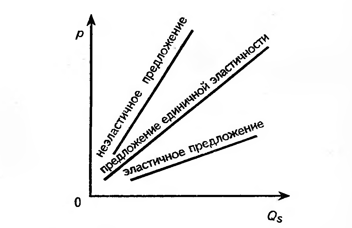
The proposal could be:
Elastic (Es > 1);
Inelastic (Es< 1);
Characterized by unit elasticity (Es =1);
Perfectly elastic (Es = infinity);
Completely inelastic (Es = 0).

Factors of supply elasticity
Elasticity of supply characterizes the magnitude of the change in the supply of a product, under the influence of factors acting on it:
Prices of other goods (including resources);
Time factor;

The degree of monopolization of the industry;
Capital mobility;
Technological features of changes in production.

Time factor
The most important factor for the elasticity of supply is the time factor, i.e. the period during which producers have the opportunity to adjust the quantity supplied to changes in price.

There are three time intervals.
Time factor for elasticity of supply
Shortest market period
The shortest market period, which is so short that producers do not have time to respond to changes in demand and prices. During this period, all factors of production are constant, which means the volume of supply is actually fixed.

Short term market period
A short-term period when production capacity remains unchanged, but the intensity of its use may change, i.e. Some factors of production become variable - raw materials, labor, etc.

Long term market period
Long-term period sufficient for change production capacity, organization of new enterprises, when all factors of production become variables.

Due to the lack of time for such a reaction, supply is completely inelastic. The rise in prices will strictly correspond to the increase in demand (the scale of the upward shift in its curve).

A large-scale example of the same kind is agricultural products. As much as the harvest is harvested, so much is collected. It will not be possible to increase production at any level of demand until next year. The justice of this situation was felt by residents of Russian cities in 1998. When import volumes fell after devaluation, prices for Russian agricultural products quickly went up. And no wonder: switching demand to domestic goods could raise prices, but not increase supply.

In the short and long periods, with an increase in demand, the volume of supply will increase, i.e. supply will acquire a certain elasticity. At the same time, the price will also rise, but to a lesser extent than the increase in demand. The differences between the short and long periods are the degree of elasticity of the curve. In the short term, it is small - by increasing the utilization of existing capacities, only a limited increase in production can be obtained. In the end, no matter how much additional raw material is supplied, the productivity of the machines processing it has its limit.

This situation is also very relevant for Russia. After liberalization foreign economic activity exports of many goods, including oil, began to grow rapidly. However, having reached a certain level (about 105 million tons per year), it froze there. Oil workers say that the limiting factor for them is the “pipe” - the throughput capacity of oil pipelines. No matter how great the foreign demand, pumps working at the limit through existing pipelines cannot pump more than a certain maximum.

But in the long term, with a favorable change in demand, there are almost no limits to increasing supply. Therefore the curve is very elastic. The response to growing demand is a large increase in production with a very moderate rise in prices. It is even possible that the price will remain constant, i.e. a perfectly elastic supply curve is realized. For example, are there any limits to beer production in Russia? If there is a need for them, you can build as many breweries as you like - the technology is simple and worked out to the smallest detail. There is an abundance of raw materials (malt) on the world market. There is also no shortage of labor in Russia. In such conditions, an increase in supply will not necessarily be associated with an increase in the price of beer.

Let's say that the initial price level covers the brewer's expenses and provides him with a decent profit. Then the response to increased demand will be a simple increase in the number of factories: similar as twins, they will have the same level of costs. Consequently, the price will suit newcomers no less than old-timers. And there will be no shortage of beer, which could push prices up. After all, each new surge in demand will lead to an expansion of capacity. So, in the absence of resource restrictions (and, as will be shown below, in the normal operation of the competition mechanism), the supply curve in the long run is very elastic, and sometimes completely elastic.

Depending on the factors affecting supply, we can distinguish different types elasticity.

Price elasticity of supply is a change in the quantity supplied of a product under the influence of a change in its price.
Price elasticity of supply can be calculated using the formula:

Elasticity of supply with respect to resource prices
According to technology changes
Elasticity of supply to changes in technology - changes in supply under the influence of changes in production technology.

Cross elasticity of supply - a change in the supply of one product under the influence of a change in the price of another product characterizes, etc.

Due to the law of supply, the price elasticity of supply is always positive.

If EpS is greater than 1, then supply is price elastic, i.e. the supply quantity reacts flexibly to price changes. In this case, the percentage change in the quantity supplied is greater than the percentage change in the price of the product.

If EpS equals 1, then the supply has unit elasticity. In this case, the percentage change in the quantity supplied is equal to the percentage change in the price of the product.

If EpS is less than 1, then supply is price inelastic. In this case, a significant change in price is required for a small change in the quantity supplied, that is, the percentage change in the quantity supplied is less than the percentage change in the price of the product.

If EpS equals 0, then supply is completely price inelastic. That is, no matter how the price of a product changes, the quantity of its supply remains unchanged.

Offers are absolutely price elastic
If EpS tends to infinity, then supply is absolutely price elastic. This coefficient is more of a theoretical model than a real one.
The degree of price elasticity of supply can be determined from the supply schedule. It should be noted that for most industrial goods, the elasticity of supply with respect to the prices of raw materials is negative, because an increase in the price of raw materials leads to an increase in the firm's costs, which, other things being equal, causes a reduction in output.

Practical significance of elasticity theory
Elasticity theory is important for determining economic policy firms importance theory and government. This is clearly seen in the elasticity example of state tax policy. Let's say the government introduces a certain (fixed) amount of tax per unit of goods, which is equivalent to shifting the supply curve S0 up to S1. Dependence of the distribution of the tax burden on the elasticity of supply (we will assume that the elasticity of demand is constant). The figure illustrates the situation before and after the introduction of the tax.

With elastic supply, the tax burden will fall mainly on the consumer, the price increase and reduction in production volume will be significant, the amount of tax will be relatively less than with inelastic supply, and society's losses will be higher. With inelastic supply, the opposite picture is observed.

Taxes and elasticity of supply
The tax amount is distributed between consumers and producers and also includes the excess tax burden, which is a deadweight cost that represents a net loss to society. Elasticity plays a big role in this case, as it allows us to determine what part of the tax is paid by entrepreneurs and what part by consumers.

In the case of elastic demand, most of the tax is paid by the producer, in the case of inelastic demand - by the consumer.
This phenomenon is easy to explain, since in the case of elastic demand, consumers, when the price of a given product rises, will tend to switch their demand to substitute goods. In the case of inelastic demand, this will be much more difficult to do.

On the contrary, if supply is elastic, most of the tax falls on consumers, and if it is inelastic, then on producers. Elasticity of supply means that producers can easily switch their resources to the production of some other good or service. In the case of inelastic supply, the reallocation of resources occurs more slowly and with great difficulty, so producers will suffer the most from the tax.
For example, change the range, technology and volume of products. It is natural that all this allows, adapting to market conditions, to shift a large share consumer tax. Conversely, producers with inelastic, “inflexible” supply are unlikely to be able to shift the tax burden to consumers. In general, the results of introducing new taxes with different degrees of elasticity of demand and supply are summarized in table.

The introduction of taxes when supply is inelastic causes completely different consequences. This is especially clear in the example of the oil export tax. In Russia, exporting oil for oil companies is much more profitable than selling it on the domestic market:
Its price abroad is significantly higher than in the domestic market;
Foreigners pay carefully and with “real” money, which cannot be said about Russian buyers, who are stuck in a quagmire of non-payments and barter.

Therefore, the supply of oil for export is actually completely inelastic and is limited only by the throughput capacity of oil pipelines.
As follows from the theory, the inelasticity of supply allows the state to collect the maximum amount tax payments. This was the case in 1993 - 1995, when export duties accounted for almost half of all budget revenues from foreign economic activity. In 1996, however, under pressure from the International Monetary Fund, the Russian government was forced to abolish the duties. Who knows, if the country had not taken this step, it might not have had to build a pyramid of GKO loans to plug holes in the budget. This means that the August crash of 1998 would not have happened. So, not only the consequences of introducing taxes, but also their abolition are deplorable.

Oil duties were abandoned, and they were remembered only after the crash of 1998, when other sources of budget replenishment almost completely dried up. The duty was set in 1999 at 2.5 Euro per 1 ton of oil, and in 2003 it reached 40 Euro per 1 ton. Inelasticity of supply turned out to be the best tax policeman. Not a single oil company has refused to export. The results exceeded all expectations. In 2000-2003 Mainly thanks to oil duties, Russia has a budget surplus - an unprecedented excess of revenues over expenses.
By interfering in market pricing, the state changes the size and direction of cash flows going from consumers to producers, i.e., in essence, it limits the freedom of consumer choice and takes on the functions that in an ideal market model the consumer should perform. As a result, economic efficiency decreases, administrative costs and bureaucratic guardianship increase. The market resists outside interference and takes revenge for it. The growth of bureaucracy, in turn, entails a number of obvious consequences, especially in Russian conditions, from distortion of information about real economic processes to increased corruption.

Sources and links
Sources of texts, pictures and videos
ru.wikipedia.org - a resource with articles on many topics, a free encyclopedia Wikipedia
abc.informbureau.com - economic dictionary of terms, events, facts and phenomena in modern Russia
youtube.com - YouTube, the largest video hosting in the world
slovarus.ru - online dictionaries search for the meaning of a word using the most popular dictionaries
be5.biz - portal educational literature for students
otvetim.info - informational portal questions and answers
all-about-investments.ru - information portal all the most interesting things in the world of finance and economics
strana-oz.ru - magazine for slow reading Domestic Notes
liga.net - information portal about everything LIGABusinessInform
yourlib.net - website for student electronic online library
malb.ru - economic portal small business step by step
ref.rushkolnik.ru - educational portal abstracts and practical assignments
ubiznes.ru - information and economic portal all about finance
bibliotekar.ru - electronic library website
aif.ru - information portal arguments and facts
avenue.siberia.net - information portal of electronic libraries
studentu-vuza.ru - educational and information portal for university students
finforum.org - financial portal Finforum
muratordom.com.ua - information portal Best home page
yaklass.ru - information site for classmates
aup.ru - administrative and management portal about the economy
studsell.com - information portal for students
bibliofond.ru - digital library Bibliofund
knowledge.allbest.ru - information portal knowledge base Allbest
web-konspekt.ru - information site to help economists
scholar.su - information site everything for the literate
50.economicus.ru - information website of the economic school
vocable.ru - website of the national economic encyclopedia
myshared.ru - information site for various presentations
Links to Internet services
google.ru - the largest search engine in the world
video.google.com - search for videos on the Internet using Google
translate.google.ru - translator from the Google search engine
yandex.ru - the largest search engine in Russia
wordstat.yandex.ru - a service from Yandex that allows you to analyze search queries
video.yandex.ru - search for videos on the Internet via Yandex
images.yandex.ru - image search through the Yandex service
video.mail.ru - search for videos on the Internet via Mail.ru
Application links
windows.microsoft.com - website of Microsoft Corporation, which created the Windows OS
office.microsoft.com - website of the corporation that created Microsoft Office
chrome.google.ru - a frequently used browser for working with websites
hyperionics.com - website of the creators of the HyperSnap screenshot program
getpaint.net - free software for working with images
Article creator
vk.com/id252261374 - VKontakte profile
odnoklassniki.ru/profile/578898728470 - profile in Odnoklassniki
facebook.com/profile.php?id=100008266479981 - Facebook profile
twitter.com/beliann777 - Twitter profile
plus.google.com/u/1/100804961242958260319/posts - profile on Google+
beliann777.ya.ru - profile on Mi Yandex Ru
beliann777.livejournal.com - blog on LiveJournal
my.mail.ru/mail/beliann777 - blog on My World @ Mail Ru
liveinternet.ru/users/beliann777 - blog on LiveInternet
beliann777.blogspot.com - blog on Blogberg
linkedin.com/profile/view?id=339656975&trk=nav_responsive_tab_profile_pic - LinkDin profile
The essence of the concept of supply-side economics supporters is to shift efforts from managing demand to stimulating aggregate supply, activating production and employment. The name “supply economy” comes from the main idea of the authors of the concept - to stimulate the supply of capital and labor. It contains the rationale for the system practical recommendations in the field of economic policy, primarily tax policy. According to representatives of this concept, the market is not only the most effective way of organizing the economy, but is also the only normal, naturally formed system of exchange of economic activity.
Like monetarists, supply-side economists advocate liberal ways of managing the economy. They criticize the methods of direct, immediate regulation by the state. And if it is necessary to resort to regulation, then this is seen as a necessary evil, reducing efficiency and tying up the initiative and energy of producers. The views of representatives of this school on the role of the state are very similar to the position of the Austro-American economist Friedrich von Hayek (1899-1992), who persistently preached free market pricing.
Recommendations in the field of tax policy
Let us dwell briefly on the recommendations of the school of supply-side economics in the field of tax policy. Representatives of this school believe that tax increases lead to higher costs and prices and are ultimately passed on to consumers. Raising taxes is an impetus for “cost-push inflation.” High taxes deter investment, investment in new technology, to improve production. In contrast to Keynes, supporters of supply-side economics argue that the tax policy of Western countries does not restrain, but increases inflation, does not stabilize the economy, but undermines incentives for production growth.
Supply-side economics advocates cutting taxes to stimulate investment. It is proposed to abandon the system of progressive taxation (recipients of high incomes are leaders in upgrading production and increasing productivity), reduce tax rates on entrepreneurship, wages and dividends. Tax cuts will increase the income and savings of entrepreneurs, lower the interest rate, and as a result, savings and investments will increase. For wage earners, tax cuts will increase the attractiveness of additional work and receiving additional earnings, incentives to work will increase, and labor supply will increase.
Laffer effect
In their reasoning, supply-side economics theorists rely on the so-called Laffer curve. Its meaning is that reducing marginal rates and taxes in general has a powerful stimulating effect on production. When rates are reduced, the tax base ultimately increases: once issued more products, then more taxes are collected. This doesn't happen right away. But in theory, broadening the tax base can compensate for the loss in tax revenue caused by lower tax rates. As you know, tax cuts were an integral element of the Reagan program.
Some other supply-side economics recommendations are worth mentioning. Since tax cuts lead to a reduction in budget revenues, it is proposed various ways“rescue” from shortages. Thus, it is recommended to cut social programs, reduce the bureaucracy, get rid of ineffective federal expenditures (for example, subsidies industrial enterprises, costs for infrastructure development, etc.). The policy of freezing social programs that are ineffective from the point of view of the ruling circles (carried out in the USA, England, France, and other countries) is based on the justifications and recommendations of supply-side economics and monetarists.
Offer- this is a set of goods, products, services offered by the manufacturer at a given price in a given period of time for sale.
There are 5 elements of a proposal:
1) resources (raw materials, materials).
2) goods for industrial purposes (equipment, machines).
3) labor (hired).
4) capital (financial and material).
5) consumer goods:
a) durable product (cars, apartments, refrigerators);
b) non-durable product (food, household chemicals);
c) services (health care, tourism, entertainment).
The composition of the offer is constantly changing, the volume is increasing, updated, including all new products (information, license, patents). And each product group generates its own special, local market.
Similar to the law of demand in a market economy, the law of supply also operates: the quantity of supply (Q) is directly dependent on the direction of change in the price level (P).
Graph 3. Law of supply.
Law of supply- This is a direct relationship between the price level and the quantity of supply.
Non-price supply factors:
level of production technology.
taxes and subsidies.
sellers' expectations on the dynamics of demand, prices and income.
number of sellers.
4. Elasticity of supply and its measurement.
Price elasticity of supply- change in the quantity of supply under the influence of price dynamics.
If a small change in price causes a significant change in quantity supplied, this is called elastic supply.
If even a very large change in price only slightly changes the quantity supplied, then such supply is called inelastic.
Elasticity is measured by the ratio of the percentage change in supply to the percentage change in price; this change is called price elasticity coefficient of supply.
To price.el.pre-i= =
If TOprice.el.pre-i1-supply is considered elastic
If TOprice.el.pre-i1 - then supply is considered inelastic
If TOprice.el.pre-i= 1 – then the unit elasticity of supply
Graph 4. Price elasticity of supply.
Factors influencing the elasticity of supply:
the value of the manufacturer's maximum possible costs for a given product.
quantity, quality, price of goods - substitutes (substitutes).
5. Interaction of supply and demand. Equilibrium price.
In the market there are sellers who set the supply price and buyers who determine the demand price, each of the market participants tries to benefit.
Salesman(manufacturer) - sell the product at the highest possible price in order to obtain the highest possible profit.
Buyer(consumer) - purchase a product at a price with maximum utility.
Under the influence of supply and demand, an equilibrium price is formed in the market, which satisfies both the buyer and the seller.
flaw
Graph 5. Equilibrium price.
When the price rises to level P 1, the desires of sellers and buyers do not coincide. Buyers will be willing to purchase the product in quantity Q1, and sellers will be able to offer it in quantity Q2.
A situation of overproduction (excess, excess) arises in the market, since the supply of goods will exceed the demand for it.
If the price is below the level of the equilibrium price P 2, then a situation of underproduction (deficit, shortage) arises in the market, since demand for the product will exceed supply.
The law of market pricing operates in the market, according to which the price in a free competitive market tends to a level at which demand is equal to supply.
Previous questions stated that costs are the main factor influencing supply.
Therefore, before deciding how much of a product to produce, a firm must analyze costs.
Costs is payment for purchased factors of production.
This indisputable truth is viewed by different economists from different positions and with different goals.
K. Marx connected the study of costs with the desire to explore the features of the exploitation of hired labor, which are reflected in value, and therefore in costs.
To produce goods, Marx believed, society must spend both living labor (necessary and surplus) and materialized labor, expressed in the cost of equipment, raw materials, fuel, etc.
These labor costs form the value of the product, which he called costs to society.
With cash proceeds after the sale of goods, the capitalist covers the costs of equipment, raw materials, fuel, energy and pays for the necessary labor. He does not pay for surplus labor.
This means that the costs incurred by the capitalist, i.e. his production costs, less costs to society (the cost of goods) by the amount of unpaid surplus labor.
It is he who is the source of profit. Therefore, For Marx, profit lies beyond costs.
In addition to production costs, Marx highlighted distribution costs, those. costs associated with the process of selling goods.
Not all circulation costs take part in the formation of the value of a product, but only that part of them that is productive, i.e. represents a continuation of the production process in the sphere of circulation (transportation, storage, packaging, etc.).
Consequently, for Marx, not all costs are price-forming.
Unlike K. Marx, modern Western economists consider costs from the point of view of a business executive.
They believe that an entrepreneur expects income from all costs without exception. On this basis, they include the entrepreneur’s profit in costs, assessing it as a payment for risk.
In their theory, production costs, including normal average profit, are called economic, or opportunity, costs.
Unlike Western economists, Marx believed that the sum of production costs (C + V) together with profit (P) forms the price of production.
In foreign literature there is a complex classification of costs.
Depending on the impact on them of an increase in production volumes, costs are divided into constants and variables.
Fixed costs F.C. (Fixed cost) – These are costs that do not depend on production volume.
These include deductions for depreciation of buildings and structures, rental payments, administrative and management expenses, etc. These costs must be paid even if the plant is shut down.
Variable costs V.C. (variable cost) - These are costs that depend on the quantity of products produced. They consist of costs for raw materials, materials, wages, etc. As production volume increases, variable costs increase.
The division of costs into fixed and variable is conditional and depends on the period for which the analysis is carried out. So, for a long period all costs are variable, because over a long period all equipment can be replaced (a new plant is bought or an old plant is sold, etc.).
The sum of fixed and variable costs forms gross or total costs TS (total cost).
Gross, variable and fixed costs can be represented graphically.
To measure the cost of producing a unit, average total categories are used. ATS (average total cost), average constants AFC (average fixed cost) and medium variable costs AVC (average variable cost).
Average costs important in determining the profitability of a firm. If the price is equal to average costs, then the firm has zero effect and there is no profit.
If the price is less than average cost, then the firm incurs losses and may go bankrupt.
If price is greater than average cost, then the firm makes a profit equal to this difference.
Average total costs are equal to total costs divided by the number of products produced:
Average fixed costs are determined by dividing total fixed costs by the number of products produced:
Average variable costs can be obtained by dividing total variable costs by the quantity produced:
Depending on the cost estimation method, accounting and opportunity costs are distinguished.
Accounting costs- this is the actual consumption of production factors for the production of a certain amount of products at their acquisition prices.
But the same resources can be used for various alternative purposes. Therefore, there are opportunity costs, or opportunity costs. For example, by organizing the production of refrigerators, an entrepreneur misses the opportunity to produce cars and receive the benefits associated with it.
Opportunity costs - This is the amount of money that can be obtained from the most profitable of all possible alternative uses of resources.
From the point of view of the receipt of funds, costs are divided into external and internal (explicit and implicit).
External costs- these are the financial costs of the company for the purchase of raw materials, equipment, transport, energy “from the outside”, i.e. from suppliers outside the enterprise.
Internal costs- these are unpaid costs for your own and independently used resource.
For example, a company uses part of the grain harvest to sow its land. The company uses such grain for its internal needs and does not pay for it.
In order to determine the maximum output that a firm can produce, marginal costs are calculated.
Marginal cost MS (marginal cost) - is the additional cost of producing each additional unit of output compared to a given output:
They are important for determining the firm's strategy. Since fixed costs are unchanged, the marginal ones are equal to the increase in variable costs (costs of raw materials, labor, etc.).
Today almost anyone developed country The world is characterized by a market economy in which government intervention is minimal or completely absent. Prices for goods, their assortment, production and sales volumes - all this develops spontaneously as a result of the work of market mechanisms, the most important of which are law of supply and demand. Therefore, let us consider at least briefly the basic concepts of economic theory in this area: supply and demand, their elasticity, the demand curve and the supply curve, as well as their determining factors, market equilibrium.
Demand: concept, function, graph
Very often one hears (sees) that such concepts as demand and quantity of demand are confused, considering them synonyms. This is wrong - demand and its magnitude (volume) are completely different concepts! Let's look at them.
Demand (English "Demand") is the solvent need of buyers for a certain product at a certain price level for it.
Quantity of demand(quantity demanded) - the quantity of goods that buyers are willing and able to purchase at a given price.
So, demand is the need of buyers for a certain product, ensured by their solvency (that is, they have money to satisfy their need). And the quantity of demand is a specific quantity of goods that buyers want and can (they have the money to do so) buy.
Example: Dasha wants apples and she has money to buy them - this is demand. Dasha goes to the store and buys 3 apples, because she wants to buy exactly 3 apples and she has enough money for this purchase - this is the value (volume) of demand.
The following types of demand are distinguished:
- individual demand– an individual specific buyer;
- total (aggregate) demand– all buyers available on the market.
Demand, the relationship between its value and price (as well as other factors) can be expressed mathematically, in the form of a demand function and a demand curve (graphical interpretation).
Demand function– the law of dependence of the quantity of demand on various factors influencing him.
– a graphic expression of the dependence of the quantity of demand for a certain product on its price.
In the simplest case, the demand function represents the dependence of its value on one price factor:

P – price for this product.
The graphical expression of this function (demand curve) is a straight line with a negative slope. This demand curve is described by the usual linear equation:

where: Q D - the amount of demand for this product;
P – price for this product;
a – coefficient specifying the offset of the beginning of the line along the abscissa axis (X);
b – coefficient specifying the angle of inclination of the line (negative number).

A linear demand graph expresses the inverse relationship between the price of a product (P) and the quantity of purchases of that product (Q)
But, in reality, of course, everything is much more complicated and the amount of demand is influenced not only by price, but also by many non-price factors. In this case, the demand function takes the following form:
where: Q D - the amount of demand for this product;
P X – price for this product;
P – price for other related goods (substitutes, complements);
I – income of buyers;
E – buyer expectations regarding future price increases;
N – the number of possible buyers in a given region;
T – tastes and preferences of buyers (habits, following fashion, traditions, etc.);
and other factors.
Graphically, such a demand curve can be represented as an arc, but this is again a simplification - in reality, the demand curve can have any most bizarre shape.

In reality, demand depends on many factors and the dependence of its value on price is nonlinear.
Thus, factors influencing demand:
1. Price factor demand– the price of this product;
2. Non-price factors of demand:
- the presence of interrelated products (substitutes, complements);
- level of income of buyers (their solvency);
- number of buyers in a given region;
- tastes and preferences of customers;
- customer expectations (regarding price increases, future needs, etc.);
- other factors.
Law of Demand
To understand market mechanisms, it is very important to know the basic laws of the market, which include the law of supply and demand.
Law of Demand– when the price of a product rises, the demand for it decreases, with other factors remaining constant, and vice versa.
Mathematically, the law of demand means that there is an inverse relationship between the quantity demanded and the price.
From a layman’s point of view, the law of demand is completely logical - the lower the price of a product, the more attractive its purchase and the greater the number of units of the product will be purchased. But, oddly enough, there are paradoxical situations in which the law of demand fails and acts in the opposite direction. This is reflected in the fact that the quantity demanded increases as the price increases! Examples are the Veblen effect or Giffen goods.
The law of demand has theoretical basis. It is based on the following mechanisms:
1. Income effect- the buyer’s desire to purchase more of a given product when its price decreases, without reducing the volume of consumption of other goods.
2. Substitution effect– the willingness of the buyer, when the price of a given product decreases, to give preference to it, refusing other more expensive goods.
3. Law of Diminishing Marginal Utility– as this product is consumed, each additional unit of it will bring less and less satisfaction (the product “gets boring”). Therefore, the consumer will be willing to continue to buy this product only if its price decreases.
Thus, a change in price (price factor) leads to change in demand. Graphically, this is expressed as movement along the demand curve.

Change in the quantity of demand on the graph: moving along the demand line from D to D1 - an increase in the volume of demand; from D to D2 - decrease in demand volume
The impact of other (non-price) factors leads to a shift in the demand curve – changes in demand. When demand increases, the graph shifts to the right and up; when demand decreases, it shifts to the left and down. Growth is called - expansion of demand, decrease – contraction of demand.

Change in demand on the graph: shift of the demand line from D to D1 - narrowing of demand; from D to D2 - expansion of demand
Elasticity of demand
When the price of a product rises, the quantity demanded for it decreases. When the price decreases, it increases. But this happens in different ways: in some cases, a slight fluctuation in the price level can cause a sharp increase(fall) in demand; in others, a change in price within a very wide range will have virtually no effect on demand. The degree of such dependence, sensitivity of the quantity demanded to changes in price or other factors is called elasticity of demand.
Elasticity of demand- the degree to which the quantity demanded changes when price (or another factor) changes in response to a change in price or other factor.
A numerical indicator reflecting the degree of such change - demand elasticity coefficient.
Respectively, price elasticity of demand shows how much the quantity demanded will change if the price changes by 1%.
Arc price elasticity of demand– used when you need to calculate the approximate elasticity of demand between two points on an arc demand curve. The more convex the demand arc, the higher the error in determining elasticity.
where: E P D - price elasticity of demand;
P 1 – initial price for the product;
Q 1 – the initial value of demand for the product;
P 2 – new price;
Q 2 – new quantity of demand;
ΔP – price increment;
ΔQ – increment in demand;
P avg. – average prices;
Q avg. – average demand.
Point price elasticity of demand– is used when the demand function is specified and there are values of the initial quantity of demand and the price level. Characterizes the relative change in the quantity demanded with an infinitesimal change in price.

where: dQ – differential of demand;
dP – price differential;
P 1, Q 1 – the value of price and quantity of demand at the analyzed point.
Elasticity of demand can be calculated not only by price, but, for example, by the income of buyers, as well as by other factors. There is also cross elasticity of demand. But we will not consider this topic so deeply here; a separate article will be devoted to it.
Depending on the absolute value of the elasticity coefficient, the following types of demand are distinguished ( types of elasticity of demand):
- Perfectly inelastic demand or absolute inelasticity (|E| = 0). When the price changes, the quantity demanded remains virtually unchanged. Close examples include essential goods (bread, salt, medicine). But in reality there are no goods with completely inelastic demand for them;
- Inelastic demand (0 < |E| < 1). Величина спроса меняется в меньшей степени, чем цена. Примеры: товары повседневного спроса; товары, не имеющие аналогов.
- Demand with unit elasticity or unit elasticity (|E| = -1). Changes in price and quantity demanded are completely proportional. The quantity demanded grows (falls) at exactly the same rate as the price.
- Elastic demand (1 < |E| < ∞). Величина спроса изменяется в to a greater extent than the price. Examples: goods that have analogues; luxuries.
- Perfectly elastic demand or absolute elasticity (|E| = ∞). A slight change in price immediately increases (decreases) the quantity demanded by an unlimited amount. In reality, there is no product with absolute elasticity. A more or less close example: liquid financial instruments traded on an exchange (for example, currency pairs on Forex), when a small price fluctuation can cause a sharp increase or decrease in demand.
Sentence: concept, function, graph
Now let's talk about another market phenomenon, without which demand is impossible, its inseparable companion and opposing force - supply. Here we should also distinguish between the offer itself and its size (volume).
Offer (English "Supply") - the ability and willingness of sellers to sell goods at a given price.
Supply quantity(volume supplied) - the quantity of goods that sellers are willing and able to sell at a given price.
The following are distinguished: types of offer:
- individual offer– a specific individual seller;
- general (aggregate) supply– all sellers present on the market.
Suggestion function– the law of dependence of the quantity of supply on various factors influencing it.
– a graphical expression of the dependence of the quantity of supply for a certain product on its price.
In simplified terms, the supply function represents the dependence of its value on price (price factor):

P – price for this product.
The supply curve in this case is a straight line with a positive slope. The following linear equation describes this supply curve:
![]()
where: Q S - the amount of supply for this product;
P – price for this product;
c – coefficient specifying the offset of the beginning of the line along the abscissa axis (X);
d – coefficient specifying the angle of inclination of the line.

A linear supply graph expresses a direct relationship between the price of a good (P) and the quantity of purchases of that good (Q)
The supply function, in its more complex form that takes into account the influence of non-price factors, is presented below:
where Q S is the quantity of supply;
P X – price of this product;
P 1 ...P n – prices of other interrelated goods (substitutes, complements);
R – availability and nature of production resources;
K – technologies used;
C – taxes and subsidies;
X – natural and climatic conditions;
and other factors.
In this case, the supply curve will have the shape of an arc (although this is again a simplification).

In real conditions, supply depends on many factors and the dependence of supply volume on price is nonlinear.
Thus, factors influencing supply:
1. Price factor– the price of this product;
2. Non-price factors:
- availability of complementary and substitute products;
- level of technology development;
- quantity and availability of necessary resources;
- natural conditions;
- expectations of sellers (manufacturers): social, political, inflation;
- taxes and subsidies;
- type of market and its capacity;
- other factors.
Law of supply
Law of supply– when the price of a product rises, the supply for it increases, with other factors remaining constant, and vice versa.
Mathematically, the law of supply means that there is a direct relationship between the quantity supplied and the price.
The law of supply, like the law of demand, is very logical. Naturally, any seller (manufacturer) strives to sell their goods at a higher price. If the price level on the market increases, it is profitable for sellers to sell more; if it decreases, it is not.
A change in the price of a product leads to change in supply. This is shown on the graph by movement along the supply curve.

Change in supply quantity on the graph: movement along the supply line from S to S1 - increase in supply volume; from S to S2 - decrease in supply volume
Changes in non-price factors lead to a shift in the supply curve ( changing the proposal itself). Expansion of offer– shift of the supply curve to the right and down. Narrowing the offer– shift left and up.

Change in supply on the graph: shift of the supply line from S to S1 - narrowing of supply; from S to S2 - sentence extension
Elasticity of supply
Supply, like demand, may vary to varying degrees depending on changes in price and other factors. In this case, we talk about the elasticity of supply.
Elasticity of supply- the degree of change in the quantity of supply (the quantity of goods offered) in response to a change in price or other factor.
A numerical indicator reflecting the degree of such change - supply elasticity coefficient.
Respectively, price elasticity of supply shows how much the quantity supplied will change if the price changes by 1%.
The formulas for calculating the arc and point price elasticity of supply (Eps) are completely similar to the formulas for demand.
Types of elasticity of supply by price:
- perfectly inelastic supply(|E|=0). A change in price does not affect the quantity supplied at all. This is possible in the short term;
- inelastic supply (0 < |E| < 1). Величина предложения изменяется в меньшей степени, чем цена. Присуще краткосрочному периоду;
- unit elastic supply(|E| = 1);
- elastic supply (1 < |E| < ∞). Величина предложения изменяется в большей степени, чем соответствующее изменение цены. Характерно для long term;
- absolutely elastic supply(|E| = ∞). The quantity supplied varies indefinitely with an insignificantly small change in price. Also typical for the long term.
What is noteworthy is that situations with completely elastic and completely inelastic supply are quite real (unlike similar types of elasticity of demand) and occur in practice.
Demand and supply “meeting” in the market interact with each other. With free market relations without strict government regulation, they will sooner or later balance each other (a French economist of the 18th century spoke about this). This state is called market equilibrium.
– a market situation in which demand is equal to supply.
Graphically, market equilibrium is expressed market equilibrium point– the point of intersection of the demand curve and the supply curve.
If supply and demand do not change, the market equilibrium point tends to remain unchanged.
The price corresponding to the market equilibrium point is called equilibrium price, quantity of goods - equilibrium volume.

Market equilibrium is graphically expressed by the intersection of the demand (D) and supply (S) schedules at one point. This point of market equilibrium corresponds to: P E - equilibrium price, and Q E - equilibrium volume.
There are different theories and approaches explaining exactly how market equilibrium is established. The most famous are the approach of L. Walras and A. Marshall. But this, as well as the cobweb-like model of equilibrium, a seller’s market and a buyer’s market, is a topic for a separate article.
If very short and simplified, then the market equilibrium mechanism can be explained as follows. At the equilibrium point, everyone (both buyers and sellers) is happy. If one of the parties gains an advantage (the market deviates from the equilibrium point in one direction or another), the other party will be unhappy and the first party will have to make concessions.
For example: price above equilibrium. It is profitable for sellers to sell goods at a higher price and supply increases, creating an excess of goods. And buyers will be unhappy with the increase in the price of the product. In addition, competition is high, supply is excessive and sellers, in order to sell the product, will have to reduce the price until it reaches an equilibrium value. At the same time, the volume of supply will also decrease to the equilibrium volume.
Or other example: the volume of goods offered on the market is less than the equilibrium volume. That is, there is a shortage of goods on the market. In such conditions, buyers are willing to pay a higher price for a product than the price at which it is sold in this moment. This will encourage sellers to increase supply while simultaneously raising prices. As a result, the price and volume of supply/demand will reach an equilibrium value.
In essence, this was an illustration of the theories of market equilibrium of Walras and Marshall, but as already mentioned, we will consider them in more detail in another article.
Galyautdinov R.R.
© Copying of material is permissible only if a direct hyperlink to